This document summarizes my notes for the XES-15 Jurassic tank run. Its goal is to save time for future runs. Indeed, realizing a JT experiment is time-consuming: XES-15 design started in August 2014, the experiment run was in February-May 2015 and I hope to finish the stratigraphic sections this June. My implication was sparse from September to December 2014 and became close to 100% of my time in January 2015. One has however to keep in mind that many technical/complex tasks were realized by Jim Mullin and Chris Ellis and are not specified in this document. You can use this document together with the XES basin operator manual.
1. Principle of XES-15 and design
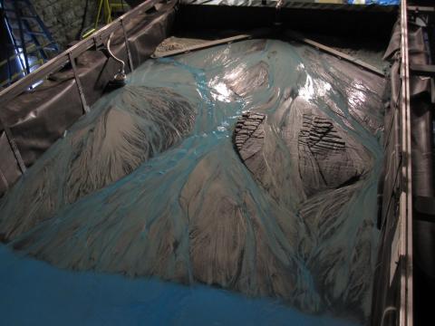
The aim of XES-15 was to study the influence and competition of tectonics and sedimentation on river path selection. To have such configuration, in addition to a main, constant sediment source, I needed a relative uplift and a secondary source of sediment. The second sediment source was integrated to the facility and is still usable for future runs. The uplift was a little trickier to create because the bottom of the Jurassic tank can only subside. Therefore, this uplift was only relative: the ocean was subsiding faster than the anticline area (see below). The rest of the basement was subsiding at a faster rate than the ocean to create accommodation space.
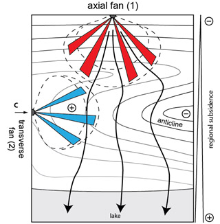
Fig1: XES-15 design
Chris Ellis has created a useful excel spreadsheet to prepare JT runs (final spreadsheet in the basin control folder). We used it a lot. It is a geometric model that fills the JT hexagonal cells one by one using alluvial slope, sediment discharge, ocean elevation and the basement evolution. It takes into account the compaction but only works for one sediment source. It will give you information like sediment thickness and shoreline evolution. You can use the spreadsheet to test and adjust your design scenario. It is powerful because you can use it to generate two important files for any JT run: the basin control file and the profile file.
Fig2: Jim Mullin on ISIS computer (left) and JT computer (right), to the left of JT computer are the fusible that control the hexagons subsidence.
The basin control program is located on the ISIS computer and controls two things: the ocean elevation and the sediment of the main sediment source. The second sediment source is controlled manually but you can connect it to an I/O switch so it is turned on and off simultaneously with the main source. Water discharges are controlled manually and need to be readjusted whenever a sources is activated (see the run section for further details). The profile file controls the subsidence of the gravel. It needs to be loaded on the JT computer in a special format so Jim’s program can read it. The profile file specifies the target elevation of the gravel layer every given interval (we choose 60 min). Jim’s program will try its best to make it happen but you will have to help it (see later).
2. Preparing the basement (gravels and pucks)
The basement is composed of gravels that lay over a honeycomb of hexagons. The first thing to do is to think carefully about the geometry of the subsidence pattern, i.e. if the slopes are too steep the gravels will slide too much and produce uncontrolled subsidence pattern. For example, on experiments where slopes were nearly vertical, the gravel were stabilized with a board. You can check cross sections of previous experiment and see how different than expected slopes are. For the XES-15 experiment, we did not place a board but expected the side of the anticline to slide a little and entrain the top of the anticline. To compensate for that, we add a minimum drop (Mindrop) of 1 mm every hour to the subsidence of each cell in the basin. Accordingly, this Mindrop was also included into the ocean elevation. A membrane is put over the gravels during the experiment. Make sure this membrane can stretch enough according to your subsidence pattern. If it is too rigid, it may tear apart, pull up the sediments or push down the gravels. The membrane I used was a 2 mm thick (1 mil) EPDM membrane. You can buy it at Roof Depot for 500 $. Be careful: one membrane from Roof Depot has seams about every two meters. It will stretch differently along these seams and might induce shearing between the membrane and the sediments. You might have to look for a different type of membrane according to your subsidence pattern.
Once the gravels are inside the basin, you will have to set up the pucks. This pucks are the heart of the JT system: when properly used, they communicate the elevation of the gravel layer to the JT program that can react accordingly. If you mess them up you have no control over subsidence. The pucks are located inside plastic boxes on the window side of JT. Jim M. has written a document about how to set them up together with the blue plastic antifriction sheets. Basically there is one puck per cell and you can add a couple of extra control puck to check particular area of the experiment (usually area with the steepest slopes). The pucks are labelled according to the coordinate of the cell they refer to. CHECK THAT IT IS THE CASE BEFORE PUTTING THE MEMBRANE. The pucks are going to slide with the gravels. If you don’t set them properly they will slide too much, give you the elevation of neighbor cells and make the JT program go crazy. In steep area, the pucks are therefore set a little upslope in the opposite direction they are expected to slide. There is a description of the puck set-up for XES-15 in the log file. Once the pucks are set up, cover with the membrane.
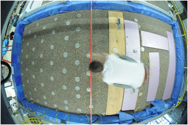
Fig3: Set-up of the pucks after the blue plastic antifriction sheets
Gravel and pucks procedure:
- Load gravel into the basin from the storage area using the gravel recirculation system :
- use garden hoses to make the gravel slide into the collecting pipes or sluice line (open river water valve beforehand)
- open the ‘basin’ valve on the mezzanine above the water control panel
- open the Venturi valve below the gravel tank in the basement level
- turn on the blue pump next this tank).
- Shovel gravels and make it even (you want to set the gravel layer an inch or two higher the initial condition of the run)
- Jim used the cart to level the surface, previous runs used a big board that two persons had to slide from the sides
- Set the pucks, use Jim’s document (XES basin operator manual)
- Level the surface once again
- Draw down the gravel to your initial conditions
- Put the membrane (You will need at least 4 peoples; it is way easier when the membrane is folded according to the basin dimensions beforehand; ask Jim M. or Chris E.)
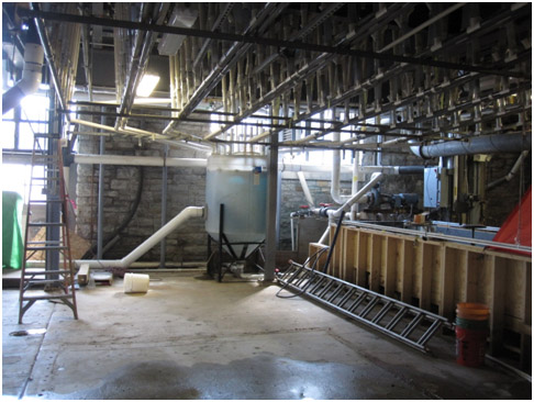
Fig4: Sluice lines and gravel recycling tank.
3. Filling of the basin (drainage layer, sediments)
Your basin is going to be filled with sediment of course, but before even starting that you need to put the drainage layer. This layer will help to drain the water out of the sediment before analyzing the stratigraphy. Usually it is a 50 mm-thick layer of ‘microfine’ sand. Ask Sara Mielke or Ben Erickson to order about 1,500 kg of microfine. The sand must be stored dry in one or two super-sacks and will be introduced using a pipe connected to the lower deck (upper right of Fig5). You need help to do that but you can shovel the sand yourself afterward. Do not step on the membrane to avoid damage, use Styrofoam pieces to move around the sand. In area where you suspect the water will be trapped, add tubes to syphon water out at the end of the run (see XES basin operator manual).
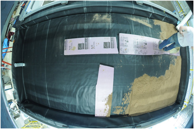
Fig5: Drainage layer filling
Finding the sediments recipe was just a nightmare for me. I hope you can reuse mine… At the end, I used a mix close to what is sometimes used in delta basin. The mix (see Table1) is composed of sand (70% volume) and Asbury ACFM2 coal (30% volume). A tiny fraction of TiO2 is added (28 g/liter of mix). This TiO2 mixes with the water and gives a milky color to the rivers, which gives a better contrast for picture analysis. The mix may be ‘white’ or colored and can be changed according to the design of the run. The ‘white’ sand is Agsco 100-140 silica sand (d50 ~ 130 μm) and the colored sand can be order on this website: http://www.kwikcolorsand.com/ (note: if you use blue dye to color the water, using blue sand is prohibited to avoid problem in the picture analysis). Density of the coal (anthracite) is 1.5 and the sand is 2.65. For XES-15, I used a colored to white sand ratio of .15 (over the sand fraction, not over the whole mix). The colored sand has slightly different properties than the plain sand. It must be washed with JetDry (ask Sara M.; 8 cups on a metal pan half-filled with water; fill ¾ with sand and mix thorefully; put in the oven and let dry for a couple of day). I had a lot a leftover from XES-15. Check around the oven if there is still some in large garbage pans.
|
Ingredient |
Coal |
Sand |
TiO2 |
Colored Sand |
|
quantity (lb) |
1 Bag + 32.5 lb |
6 bags + 17 lb |
8 lb |
1 bag |
|
total (kg) |
37 kg |
143.9 kg |
3.64 kg |
22.5 kg |
Table 1: Mix for one load of sediments (.13 m3). You can put about 4 loads in hoper 1 and 3 loads in hoper 2. If you don’t need colored sand, replace by 1 bag of sand.
You can place orders with help from Sara Mielke. I suggest that you check in the Quonset hut if there are some leftovers from previous experiment. Expect a couple of weeks for shipping. Once the coal and sand are at SAFL, STORE THEM IN A DRY PLACE! Wet sediments will clogged the sediment feeder, potentially ruin your experiment and give you a hard time cleaning your supply line.
Here are two calibration curves available for the Sediment feeder 1 and 2 used for XES-15, respectively called qs1 and qs2. You probably will have to check these calibrations yourself. Use a watch and a graduated cylinder for that.
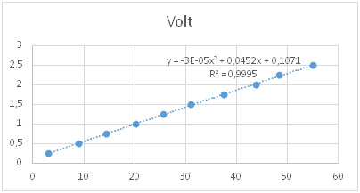
Fig6: Qs 1 voltage as a function of sediment feed rate (l/hour). The fit was used by Chris E. in the basin control program to automate it.
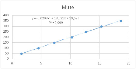
Fig7: Qs 2 mute as a function of sediment feed rate (l/hour). Numbers had to be entered on qs2 screen (set on manual).
During the run, sediment sources are connected to the basin with plumbing adapted to their water discharge (checking that before starting the run is wise, especially if you will run with high water discharge). The highest water discharge you can get is 1.3 LPS (~ tap water discharge); it is huge and will give a lot of momentum to your flow. When we tried 1.1 LPS in qs1 for XES-15, the sediment started to prograde very fast, a lot faster than what we expected… In the basin, the sediment source are hooked up to a gravel baskets. These baskets help distributing the flow and preventing the formation of too large scours.
4. Mixing sediments
The mixing has to be done before and during the run. Try to anticipate and coordinate with weather forecast and students’ availability. It is the dirtiest procedure (because of coal and TiO2), don’t wear nice clothes when you mix.
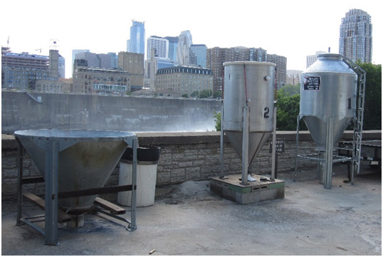
Fig8: From left to right: transfer hoper and hopers 2 and 1 (connected to qs2 and qs1, respectively)
Procedure:
-Check the weather first, a rainy day will wet the sediments.
-Use respirator, gloves, and glasses and mix the sediments outside. Ask Ben E. where the best place is. You need to do that with somebody who can use the forklift. A student of the shop (Kyle?) can help.
-Usually mix half of the coal and half of the sand for a few minutes, then add the other half of each. Let mix for a few minutes (until it looks thoroughly mixed).
- Sift in TiO2. Make sure to have a mixer cover handy to keep the dust down.
-Raise mixer above transfer hopper and dump sediment. MAKE SURE FORKLIFT FORK IS IN THE SLEEVE ON THE MIXER. WE DON’T WANT IT TO FALL AND BREAK!!
-Once transfer hopper is ~3/4 full, use fork extensions to lift by C-channel on transfer hopper and move up to one of the large hoppers on lower deck.
-CAREFULLY RAISE TRANSFER HOPPER ABOVE AND DUMP. THIS IS DANGEROUS LIFTING THAT MUCH WEIGHT THAT HIGH WITH THE FORKLIFT!! MAKE SURE NO ONE IS NEARBY.
-IF IT STARTS TO RAIN, QUICKLY MOVE EVERYTHING INSIDE THE QUONSET. THE SEDIMENT (ESPECIALLY MIXED SEDIMENT) CANNOT GET WET.
-Fill hopper on lower deck until about 1 foot from the top. Leave any extra in the transfer hopper and store in the Quonset hut.
5. Mixing 4 gallons of dye
Dye allows to make nice picture and extracting river position. It is absolutely necessary to have good data. I needed about one gallon of dye every 10-15 hours per sediment feeder. I used about 24 gallons for my experiment.
Warning:
Dye is non-threatening but gets everywhere (skin + clothes). Make sure to wear appropriate clothes and eventually bring a towel to get a shower after mixing. Inform peoples like Ben or Dick about what you are about to do. They will give you other instructions.
What you need:
- A nice space, above a grid with one (or two) hoses to clean the tools as you mix. Next to the landscape facility in the basement is nice.
- Black bucket with cap; funnel, red helix: you will find these in the delta basin cabinet.
- An old, not nice, drill (to attach to the helix); a garbage can or orange bucket with two garbage bags: place one in the bucket and one above to cover the bucket; gloves; eventually a white suit to protect your clothes, you can tape your sleeves to the gloves to protect your wrists (and you will look like a Fukushima or Ebola guy). Find these in the shop.
- One dose of dye powder (name?) in small plastic container stored in the dye cabinet. Ask either Ben or Dick to open it and make sure that there is enough dye for the future. If not ask them to order some.
- 4 gallons of water (tap water is fine) in 4 plastic or glass bottles.
OK, ready?
- Place the dye dose into the garbage can and cover it with the second plastic bag to avoid accident (the dye powder is very volatile and will stay forever in one spot: you don’t want that)
- Go to your nice spot
- Put 2 gallons of water in the black bucket
- Gently pour the dye in the water (tip: slide the top plastic bag with the plastic container from one bucket to the other to avoid blowing dye on your face).
- Cover the black bucket with the white cap. Put the helix attached to the drill. Tip: cover with plastic bag to protect you from splashing (be careful to not pinch the plastic into the drill).
- Mix thoroughly for 3 minutes (make sure there is no deposition in the bottom of the bucket: this will save you trouble during your experiment).
- Take out the helix and clean the tools. Put two more gallons of water (use the funnel) and start mixing again for another 3 minutes.
- Use the funnel to pour the liquid dye in the bottle (needless to say: do that above the grid and take a deep breath).
- Put a cap above the bottles (to limit evaporation) and store the bottles in oranges buckets.
- Clean the space and take out the trash.
Congratulations you are done: count the amount of dye drops on you and you may (or not) make fun of others.
6. Ocean control system
It is an important part of the Jurassic tank facility. It was crucial for XES-15 because it was controlling the base-level and therefore the relative uplift rate of the anticline. Once the membrane and drainage layer are in place, start flooding the basin. You can then set the ‘ocean sucker’. This system connects your ocean to a weir mounted on a motor. Ultimately, the height of the weir will control the ocean level. This weir is moved by the basin control program. Some water is constantly added into the line. This extra flow helps rising the ocean level when too low and just flows over the weir when too high. A side glass and a cylinder with a sonar sensor inside are also connected to the ocean control system. They allow measuring the ocean elevation at any time and it is recommended to check once in a while that they match. These systems are controlled by suction lines. Make sure that these lines work properly.
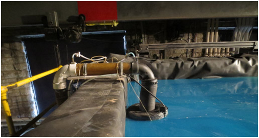
Fig9: ‘Ocean sucker’. The black tube is the suction line that remove the scum floating at the ocean surface.
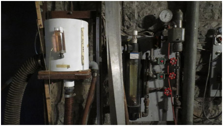
Fig10: Computer-controlled weir (left) and water inflow (right, bottom red valve)
7. Starting the run and daily procedure / JT-sitting
If you have accomplished all steps listed above, congratulations! You have finished an important part of the job. The more carefully you have done it, the more chances the run has to go smoothly. Well... it’s all relative.
You should now have:
- A basin with a gravel layer at the elevation you want and pucks correctly set-up. It is covered by a membrane and a drainage layer (remember that in the experimental world, your basement is the top of the drainage layer and not the gravel layer).
- Water in this basin at the elevation you want (read by both the side glass and the basin control program).
- One or several source of sediments (sediment feeder connected to hoper, water sourceand dye pump)
- A scanner properly calibrated and that is not going to hit anything inside or outside the basin.
- An ISIS computer with the basin control and time lapse photography set up (make sure you have enough storage to save your data, it can get filled rapidly). The timer of the basin control program must be linked to the JT computer. The JT program will therefore be the only one you need to turn on and off. This requires many remote connection between different machines. MAKE SURE THEY ARE CORRECTLY LINKED.
- A log file ready. In this file, you will record everything that happen during the run, the correspondence between the scan number and runtime, etc. This file is PRICELESS when you start analyzing the data month after the experiment.
The following is a summary of what I did every day during the run.
- Purge the pucks and check their elevation
The pucks lines must be filled with water (no air or algae inside). Before the run, the puck lines must be carefully purged and filled with water (it’s tricky so Jim M. did it). This water contains bleach and is maintained at temperature in two garbage drums located on the main floor. To prepare more water, fill the left drum with distilled water and 1/8 of a bleach cap. Let the water degasing for a couple of day before setting a syphon from the left to the right drum.
After each day of run, the pucks go through a slow purge. You have to make sure they work correctly in the morning, Jim has written a routine in the XES basin operator manual. To summarize you need to:
- Make sure there is enough water with bleach in the drums (main level)
- Stop night purge
- Manually purge the mux/wafer lines and check that is no air or algae in the tubes
- Level the upper and lower tank
- Restart scan and let the read values stabilize (especially control pucks!)
Take your time doing this, a bad reading of the pucks elevation will drive both the JT program and yourself crazy.
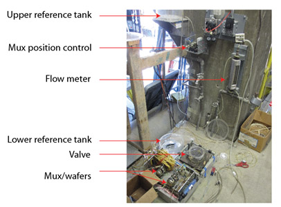
Fig11: Pucks’ mux system.
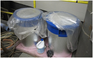
Fig12: Pucks water drums.
- Launching the experiment
Before restarting, you have to open the water on the sluice line that collect the gravels. The sluice line must be almost completely full of water (if there is not enough water, they will get clogged with gravel and the subsidence will not work). Do it while the pucks elevation are being scanned until they stabilize. Make sure the water control panel is correctly set. The pump switch must be on (green light), the inflow water must be opened and the flow coming after the head tank must be diverted to qs1 and / or qs2 depending on the run design. Also, check that the sediment feeder qs1 is on (green light).
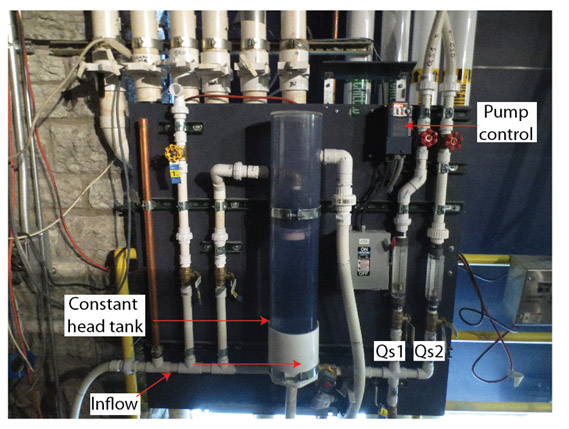
Fig13: Water control panel scheme.
Once everything is ready, follow these steps:
- Start the ‘pre-wet’ on the basin control program
- Go adjusting qs1 and qs2 water discharge to the expected values using the two red valves (Fig13)
- Check that sediments are coming out of the feeders and that the basin is wet with blue water
- Go to the JT computer and press [ctrl + F12] (it won’t work if the Array screen is still on ‘Halt Scan’)
- Adjust the pause between wafers (default is 270 seconds; during subsidence 20-30 s is OK).
You will have to redo this procedure each time you stop the experiment (to do a scan for example). In between scans, you should check several things:
- The bottle of dye is full enough and there are no bubbles flowing through the vinyl tubes
- The water discharge is correct
- The ocean control system is working and the ocean level is close (less than 1 mm) enough to the expected value (Check side glass once in a while).
- The sediment feeder is working properly (I measured sediment discharge every hour) and there is enough sediment in the hopers
- The spotlights are working correctly and the mezzanine lights are off.
- The ‘deltas’ (difference between expected and measured position of pucks) is close to zero on the JT computer.
Usually, it’s not recommended to leave the experiment for too long. If anything of the above goes wrong, you might consider stopping it, fix the problem and restart. The worst thing that can happen is the formation of a canyon that will incise the deposits. It usually occurs when the water discharge is too high or the sediment feed rate is too low…
Finally, you will also have to recycle the gravels back to the storage pile next to the experiment during the day (usually once or twice a day, depending on your subsidence rate). The procedure is similar to the once you did to fill the tank with gravels. MAKE SURE THE BASIN PIPE IS CLOSED AND THE GRAVEL PIPE OPENNED (above the water control panel), otherwise you will dump the gravels back over the deposits!
To do a scan, you need to stop the experiment and wait until the surface dries up (it takes 2 minutes). Turn of the spotlights, it is not always necessary but generally easier. From the ISIS computer, you can remotely control the XES cart computer. Go to the program called Virtual Basics, NCED data acquisition. Click on the running man to activate the program.
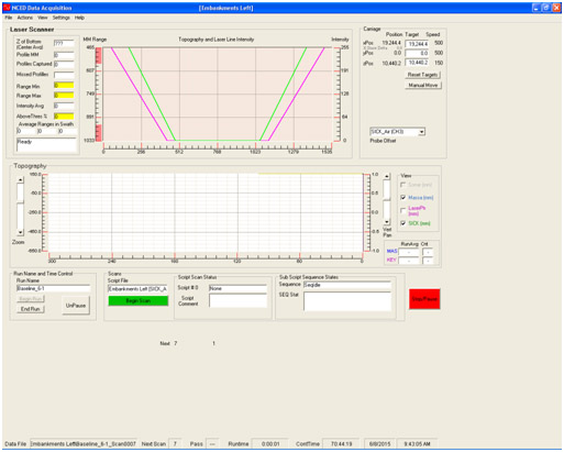
Fig14: Screenshot of the scanner acquisition program
Make sure the parameters loaded are correct (batch file and SICK parameters). Check that nothing stands in the way of the cart (all sensors on it are expensive and will take weeks to repair!). Click begin scan. The program will ask you several questions: MAKE SURE YOU UNDERSTAND THEM before saying yes. The cart will move toward the basin and stop before the wall. Check that there is room to enter (i.e. the membrane is properly folded). Click OK. The cart enters the basin and start doing several swaths. The number of swaths and their path must be adapted to the topography and the disposition of the point source (the so-called gravel baskets). Contrarily to previous runs, XES-15 was constantly subsiding and the height of the camera had to be consequently adjusted. We had to make sure the scanner was not hitting anything because of that.
Once the swaths are finished, the data acquisition program will ask you if he can get the scan out of the basin. Check again that nothing is in the way and you can click OK. The cart will go back to its home position away from the experimental basin and the gravel pile. Before restarting the experiment, PROCESS THE SWATHS TO SEE IF YOUR DATA ARE OK. If your data are bad, not even Jim can fix it afterwards... Go to the NCED sick scan processing program. Double click on the Swath log file window. Choose the swath you have just finished and click Apply then Process scan. Once the scan is finished, you can look at it on the JPEG file that opens automatically or using the Ranger Studio program. This program allows to check manually any elevation or to visualize the topography in a 3D window.
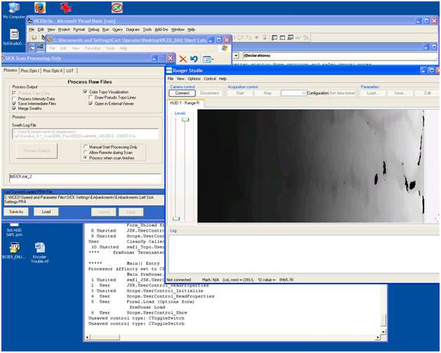
Fig15: Screenshot of the SICK scan process and Ranger Studio programs
- Stopping the experiment over night
The procedure is basically the inverse of the morning:
- Stop the run [Ctrl+F12], turn of the spotlights and make your last scan
- Turn of the pumps (dye, water, sediment feeder)
- Go to the JT program on the ‘Array’ screen
- Hit [Ctrl+F11] until you get to ‘Halt-Scan’
- Hit [Ctrl+F9], you will go to the purge screen
- You can use default to purge wafer overnight (or purge everything, 1000 times, 200 minutes between purges).
- Before leaving, don’t forget to turn off the water in the sluice lines.
8. Cutting the deposits
a) Preparation
Once the experiment is over, you need to shut down the JT program and disconnect the pucks line (there is a switch in the panel above the JT computer). Ask Jim about it. Make sure to save properly copies of the data (scans, pictures and log files) in as many external drives as you want. The next phase is to cut the deposits to analyze the stratigraphy. The expert in this domain is Dick Christopher.
Before you can cut the deposits, you need to protect and prepare them. First you need to disperse some sand (a couple of inches) on top of the deposits to protect them from collapsing or any external damage. Drain the water and put sand in the ocean too. Don’t hesitate to put more sand there as it is an area that is more likely to collapse. The sand to use is typically the same type than the drainage layer (order the same amount of ‘microfine’ sand).
Let the deposit dry for a couple of week. Install a suction line in the drainage layer in the lowest point of the basin (typically where the ocean control system was). The trick is to maintain enough moisture so that the deposits have a nice cohesion but not too much or they will flow when you cut. YOU DON”T WANT THE DEPOSITS TO DRY COMPLETELY. At this point the experience of Dick is really helpful. He will let you know if the deposits are looking good. To avoid the top of the deposits to dry too much (water flows downstream so the top gets dry more quickly), it is good to re-humidify the top of the deposits every 1-2 days with a hose connected to a mister. Do that for 10-15 minutes. Once you have a nice cohesion of the deposits, you can start cutting.
What you need:
- A box (labeled “JT cut”) stored in the mezzanine with cutting tools inside (trowel, feather duster, tubing for drying the drainage layer, a couple of shovels...)
- A plastic 50-100cm grid and blue foam boards where you can work on (see Fig. 16)
- The shoring devices (pipes with springs and wood boards to put against deposits and avoid collapsing; Fig. 16). There is also a red pipe that extend along the width of the deposits fo additional support.
- Strings to mark where the sections are going to be.
- Dirty close (you are going to ruin them).
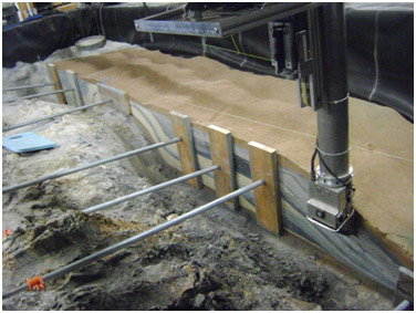
Fig. 16: Picture of the deposits being cut along a dip sections with shoring to maintain the deposits face. To the right is the camera mounted on the cart in place of the laser and camera.
If you are going to do peels (i.e. vertical slices of the deposits), you will need:
- 3m spray adhesive 77 (one per 1-2 m2 approximatively).
- Glove, mask and white painting suits
- Plastic sheets.
- A structure to maintain the plastic sheet (with tape)
- Dick to explain how it works
Before you start cutting please think carefully about your cutting plan and discuss it with peoples:
- Once you remove the sand it cannot be put back…
- Deposits 30cm along the sides are not going to be reached by the Telescan system.
- It is better to start cutting from upstream (or upslope) for stability of the pile. If you start downstream the deposits might slide and make cracks.
- Think about the orientations of the successive sections. The Telescan camera work only for dip and strikes (for a diagonal, like I [Dick] did, you will have to make a peel). On top of that, it is time-consuming to switch the orientation of the camera if you have to make multiple dip and strikes. Try to devise a plan that avoid doing it too many times…
b) Cutting procedure
First you have to program the cart to the Telescan mode. Jim (or Eric) is going to change the laser camera to a Telescan camera and enter the coordinates of your sections. You can modify it while you cut. There are two modes in the Telescan: cutting or scan. Depending on which mode you are, you need to install or remove the cutter over the camera (Fig. 17). Set up the program to cutting mode first and install the cutter on top of the camera.
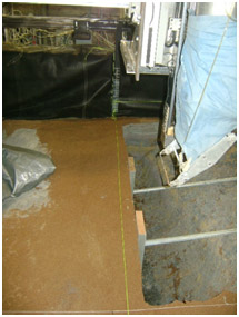
Fig. 17: Telescan system with the cutter installed on top of it.
Usually it is good to dig a 10-20 cm wide trench in front the section of interest (Fig. 18). Use strings to know the position or the laser of the cart (‘Jog mode’). DO NOT REMOVE TOO MUCH FROM THE TANK. Indeed, as you cut you have to avoid changing too much the weight distribution within the tank.
Dig by hand to get close to the section (~ 1 cm; Fig. 18). As you cut, position shoring every ~ 50 cm to protect the deposits from collapsing. The cutter is going to finish the section (Fig. 17). Set it up to 1-3 mm from the section you are aiming for. Do several pass at the beginning to get used to it.
Once you are at the desired position, clean the face with the duster. Ask Dick to show you. Remove the cutter and set the program to scan mode. Launch the program (make sure the camera has nothing in its way…), remove the shoring and put it back in the sections of interest as you scan. Check regularly on the screen that all pictures are taken, otherwise you will have to restart if one is missing (it happens sometimes, don’t know why). At the end of the pass, zip the files and eventually start the merging of the picture to create a composite section.
Then put back the cutter and set the program to the next section. Bury the trench you have done and move on to the next section…
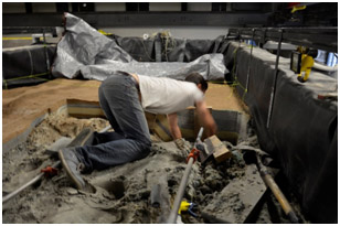
Fig. 18: Digging, exposure and burial of a section. Note that the leftover sand is kept in the tank to ensure stability of the deposits. Use as many shoring as necessary to maintain the face stable.
Once the pictures are merge, you will need to set up filter to process the pictures. Jim is the one to ask how to do. Make sure you keep a copy of all the raw data safe if you ever want to reprocess them.